Abstract: The Criticality of Multi-Modal Perception
Autonomous navigation in extraterrestrial environments is defined by an unbreakable physical constraint: the speed of light. With Earth-Mars communication latencies ranging from 4 to 24 minutes, real-time teleoperation is impossible. To survive, a rover must possess a robust Rover Perception architecture.
Rover perception is not merely the collection of images; it is the transformation of raw sensory data into a semantic and geometric understanding of the surrounding environment. This process must occur on-board, often on resource-constrained processors (such as the radiation-hardened RAD750).
Navigation reliability depends on Sensor Fusion: the algorithmic integration of exteroceptive sensors (which look outward, like Cameras and LiDAR) and proprioceptive sensors (which look inward, like IMUs). This article analyzes the engineering behind these digital “eyes” and the mathematics that allow them to work in unison.
1. Stereo Vision: Depth Perception Through Triangulation
Stereo vision remains the pillar of Rover Perception for current Martian missions, including NASA’s Perseverance and Curiosity. Unlike a single camera, which flattens the world into 2D, stereo vision emulates human binocular vision to calculate depth.
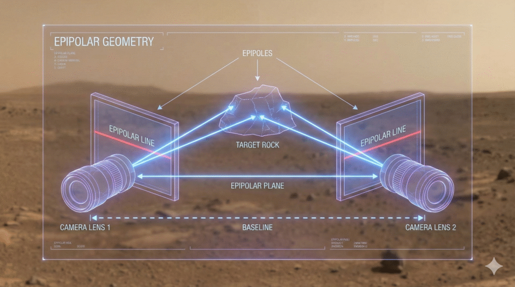
The Principles of Epipolar Geometry
The system uses two cameras separated by a known horizontal distance, called the baseline. When the onboard computer analyzes the left and right images, it searches for pixel correspondences between the same object.
The difference in an object’s horizontal position between the two images is defined as disparity. Depth Z is calculated inversely to disparity according to the formula:
Z = \frac{f \cdot B}{d}Where f is the focal length, B is the baseline, and $d$ is the disparity.
Hardware Implementation & Limitations
Perseverance’s NavCams offer a 20-megapixel resolution, allowing for the generation of high-fidelity 3D meshes. However, passive stereo vision has critical limits:
- Texture Dependence: It performs poorly on uniform terrain (smooth sand) where finding pixel correspondences is difficult.
- Lighting Conditions: It requires ambient lighting. In shadowed regions or at night, the system becomes blind without artificial illuminators.
2. LiDAR (Light Detection and Ranging): Precision Point Clouds
While stereo vision estimates depth, LiDAR measures it directly. This active sensor emits laser pulses and calculates distance by measuring the signal’s Time of Flight (ToF).
Generating Dense Point Clouds
The result of a LiDAR scan is a Point Cloud: a set of millions of vectors in 3D space.
- Operational Advantage: Unlike cameras, LiDAR is independent of ambient light. This is crucial for missions like VIPER (NASA), destined for permanently shadowed regions (PSRs) on the Moon.
- Spatial Resolution: Modern 3D LiDARs can scan 360 degrees, creating instantaneous volumetric maps (Voxel Grids) that allow navigation software to identify negative obstacles (craters) or positive obstacles (rocks) with millimeter precision.
Why Isn’t LiDAR on Every Rover?
Despite its precision, LiDAR has historically presented disadvantages in terms of SWaP (Size, Weight, and Power). Rotating mechanical parts are failure points in environments rich in abrasive dust like Mars. However, the advent of Solid-State LiDAR (with no moving parts) is shifting this paradigm for future Rover Perception missions.
3. IMU (Inertial Measurement Unit): The Proprioceptive Anchor
If cameras and LiDAR are the “eyes,” the IMU is the rover’s inner ear (vestibular system). It is a fundamental proprioceptive sensor for estimating position when visual sensors fail (e.g., Visual Blackout due to dust storms or occlusion).
Components and Functionality
A space-grade IMU typically combines:
- Accelerometers (3 axes): Measure linear acceleration (including gravity).
- Gyroscopes (3 axes): Measure angular velocity (rotation rate).
The Drift Problem
The IMU operates at high frequency (often >200 Hz), much faster than cameras. However, it suffers from Drift. To obtain position, accelerometer data must be integrated twice (from acceleration to velocity, from velocity to position).
x(t) = \iint a(t) \, dt^2
Any small sensor bias error accumulates quadratically over time, rendering the IMU unreliable over long distances unless “corrected” by external data.
4. The Core Architecture: Implementing Sensor Fusion
The true magic of Rover Perception lies in data fusion. No single sensor is perfect: vision is precise but slow and light-dependent; the IMU is fast but prone to drift; LiDAR is precise but energy-expensive.
The industry-standard algorithm for fusing these inputs is the Extended Kalman Filter (EKF).
How the EKF Works
The filter operates in a continuous two-phase cycle:
- Prediction (IMU Phase): The rover estimates its new position based on internal kinematics (IMU/Wheel Odometry). Position certainty decreases (covariance increases).
- Update (Vision/LiDAR Phase): As soon as visual data is available (e.g., Visual Odometry), the filter corrects the predicted estimate. Position certainty increases (covariance decreases).
Python Example: Simplified Sensor Fusion Logic
Here is Python pseudocode conceptually illustrating this cycle in a navigation system:
class RoverKalmanFilter:

    def __init__(self):

        self.state_estimate = 0.0  # Initial position

        self.error_covariance = 1.0 # Initial uncertainty

    def predict(self, imu_data, dt):

        """

        Prediction Phase: High frequency (e.g., 200Hz)

        Uses IMU to update the estimate, but uncertainty grows.

        """

        # Simplified velocity integration

        self.state_estimate += imu_data['velocity'] * dt

        # Add process noise (Drift) to uncertainty

        process_noise = 0.1

        self.error_covariance += process_noise

        return self.state_estimate

    def update(self, visual_odom_data):

        """

        Update Phase: Low frequency (e.g., 1-10Hz)

        Uses Vision to correct IMU drift.

        """

        # Calculate Kalman Gain (how much to trust the new measurement)

        measurement_noise = 0.5 # Typical camera error

        kalman_gain = self.error_covariance / (self.error_covariance + measurement_noise)

        # Correct the estimate based on the difference between expected and measured

        innovation = visual_odom_data['position'] - self.state_estimate

        self.state_estimate += kalman_gain * innovation

        # Reduce uncertainty (Covariance collapses)

        self.error_covariance *= (1 - kalman_gain)

        return self.state_estimate
5. Case Study: Perseverance vs. VIPER
The Rover Perception architecture is dictated by the mission environment.
- Perseverance (Mars): Utilizes a sophisticated Visual Odometry system. The rover captures images while moving, tracks salient features in the terrain, and calculates relative motion. Thanks to dedicated FPGA processors, it can process these maps and execute autonomous navigation (“AutoNav”), covering over 100 meters per Sol without human intervention.
- VIPER (Moon): Destined for the Nobile Crater, it must face perpetual darkness. Here, stereo vision is useless without its powerful LED headlights. The rover will rely critically on the fusion of IMU data and visual odometry assisted by active light to avoid getting lost in an environment lacking GPS and filled with deceptive shadows.
Conclusion
Rover Perception is not about choosing the “best sensor,” but about creating a redundant architecture. The integration of Stereo Vision for semantic context, LiDAR for precise geometry, and IMUs for high-frequency stability allows modern rovers to traverse terrains that human pilots would find challenging even remotely.
The future lies in neuromorphic cameras (event-based cameras) and edge AI computing, which will allow rovers to perceive motion with the biological efficiency of an insect, drastically reducing power consumption and increasing decision-making autonomy.
Would you like me to develop a specific deep-dive article on “Visual Odometry Algorithms: From Features to Trajectory” to link internally to this piece?

Lascia un commento