The 2.7 Billion Paradox
Imagine designing the most sophisticated vehicle ever built by humanity, a mobile laboratory costing 2.7 billion, destined to search for traces of ancient life on another planet. Now, imagine having to pilot it using a “brain” less powerful than the one on your wrist right now.
This is the reality of aerospace engineering. NASA’s Perseverance rover operates on a BAE Systems RAD750 processor. It is a Rad-Hard component (resistant to ionizing radiation) based on PowerPC architecture from the late 90s, with a clock speed of just 200 MHz. To put it brutally: your smartphone chip is hundreds of times faster.
In this scenario, software efficiency isn’t an academic luxury; it is an unbreakable physical constraint. Autonomous navigation doesn’t just mean drawing a straight line on an empty map. It means surviving a “mathematical maze” of slippery slopes, sharp rocks (called ventifacts), and soft sand traps, all while having to conserve every single CPU cycle and watt of energy.
Since direct control from Earth is impossible due to the communication delays inherent in orbital mechanics (a challenge we analyzed in detail in our article on The 20-Minute Lag), the rover is alone. It must make life-or-death decisions autonomously.
This is where pathfinding algorithms come into play. They are not just lines of code; they are the rover’s true pilots. In this article, we will analyze the “decision engine” that drives Martian exploration, comparing two giants of graph theory: A* (A-Star), the deterministic standard for global planning, and D *Lite, the master of dynamic navigation and real-time replanning.
Seeing the World in Math: Cost Maps and Occupancy Grids
Before an algorithm like A* or D* Lite can calculate a trajectory, the rover must translate the geological chaos of Mars into an ordered data structure. Computers don’t “see” rocks, dunes, or craters; they see numerical matrices.
The process begins with Perception. Navigation cameras (NavCams) and LiDAR sensors (if present, or simulated via Stereo Vision) generate a 3D “Point Cloud.” However, planning a path directly on millions of raw 3D points would be computationally prohibitive for the RAD750 CPU. The solution is the discretization of the environment into a 2D grid, known as an Occupancy Grid.
The Binary Limit: The Occupancy Grid
In its simplest form, an Occupancy Grid is a binary map that divides the surrounding terrain into fixed-size cells (e.g., 20×20 cm per cell).
- 0 (Free Space): The cell is empty and safe.
- 1 (Occupied Space): The cell contains an insurmountable obstacle.
While efficient in terms of memory, this binary approach is often insufficient for space exploration. It fails to distinguish between flat, solid ground (bedrock) and a soft sand dune that could trap the wheels. To a rover, both are “free” (there is no wall in front), but one is deadly.
The Nuance: Traversability Cost Maps
To overcome binary limits, modern systems like Perseverance’s AutoNav use Cost Maps. Instead of 0 or 1, each grid cell contains an integer value (usually 0 to 255) representing the Traversability Cost.
This cost is a function derived from three critical physical variables:
- Slope: The inclination of the terrain. Beyond 30°, the risk of tipping becomes unacceptable.
- Roughness: The variance in terrain height within the cell. It indicates how “bumpy” the surface is.
- Step Hazard: The presence of sudden negative drops (holes) or positive rises (high rocks) that could strike the rover’s belly pan.
The “Lethal” vs. “High Cost” Dilemma
The distinction between a cost of 254 (Lethal) and a high cost (e.g., 200) is what makes autonomous navigation intelligent.
- A Lethal Cost (like a vertical wall) acts as a wall: the algorithm cannot plot a path through that cell.
- A High Cost (like a deep sand field, similar to what trapped the Spirit rover at “Troy” in 2009) is mathematically traversable, but the algorithm will avoid it unless it is the only possible option to reach the goal.
It is on this matrix of numbers—not on the spectacular images we see—that A* and D *Lite fight their battle for optimization.
A* (A-Star): The Deterministic Standard for Global Planning
If autonomous navigation has a “founding father,” it is the A* algorithm (pronounced “A-Star”). Published in 1968 by Hart, Nilsson, and Raphael, it remains the reference algorithm for pathfinding on static graphs. In the context of a Martian mission, A* is often the Global Planner: the system that decides the general route based on orbital maps before the wheels even start turning.
The Theory: Optimization via Heuristics
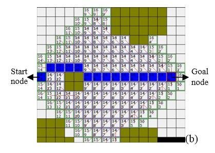
A* does not merely explore the grid blindly (as Dijkstra’s algorithm would); it is an “informed” search. It selects the path by minimizing the following cost function f(n) for each node n:
f(n) = g(n) + h(n)
Where:
- g(n) (Real Cost): The accumulated cost to travel from the starting point to the current node n. This value includes data from the Cost Map discussed above (slope, roughness, distance).
- h(n) (Heuristic Cost): An estimate of the remaining cost from n to the final goal. It is the “compass” that orients the search towards the destination.
The Compass: Choosing the Right Heuristic (h)
The efficiency of A* depends entirely on the choice of the heuristic. On Mars, topology dictates specific choices:
- Manhattan Distance (|x_1 – x_2| + |y_1 – y_2|): Standard for urban grids or 4-direction movements (North, South, East, West). It is unsuitable for rovers, as it overestimates diagonal distances in open spaces.
- Euclidean Distance (\sqrt{(x_1 – x_2)^2 + (y_1 – y_2)^2}): The “as the crow flies” distance. It is the most common heuristic for open-field space navigation since it allows movement in any direction. However, it is computationally more expensive due to the square root calculation.
- Octile / Diagonal Distance: An excellent compromise for the 8-connected grids used by rovers. It allows diagonal movements at a cost of \sqrt{2} and cardinal movements at a cost of 1.
Technical Note: To ensure A* finds the optimal path, the heuristic must be admissible (it must never overestimate the real cost). If h(n) is too aggressive, the algorithm becomes fast but inaccurate; if it is too conservative, it becomes as slow as Dijkstra.
Best Use Case: Global Planning with HiRISE
The ideal use case for A* is strategic planning on static maps.
Before a “drive,” JPL operators or onboard software download orbital images (e.g. from the HiRISE camera on the Mars Reconnaissance Orbiter). Since these maps do not change during the minutes of the drive, A* can calculate the optimal path once, ensuring minimal energy consumption.
Open Source Resources: Implementation Reference
For students and researchers looking to analyze robust implementations of A* used in real robotics, here are some Open Source references that meet industrial standards:
- ROS Navigation Stack (navfn):
The de-facto standard in terrestrial and research robotics. The navfn package within ROS (Robot Operating System) uses a highly optimized implementation of Dijkstra/A* for the Global Planner.- Repository: github.com/ros-planning/navigation
- PythonRobotics:
An academic collection of robotics algorithms. The PathPlanning section offers clear and readable implementations of A* for educational purposes.- Repository: github.com/AtsushiSakai/PythonRobotics
- NASA F Prime (F´):
Although it is a flight framework and not a pure navigation library, understanding NASA’s cFS (Core Flight System) architecture helps to understand the environment in which these algorithms must run.- Repository: github.com/nasa/fprime
The Flaw: The Cost of “Re-planning from Scratch”
If A* is so precise, why isn’t it enough? The problem arises when the map changes.
Imagine the rover, following the A* path, detects a 30cm rock via its stereo cameras that wasn’t visible from orbit. The local Cost Map changes instantly: a cell switches from “free” to “obstacle.”
A* is a static algorithm. It has no memory of past calculations. Faced with a new obstacle, it must invalidate the previous path and recalculate everything from zero (re-planning from scratch). In a complex and unknown environment, this forces the rover to stop frequently to “think,” destroying the average speed of advancement. This is where the need for dynamic algorithms enters the stage.
D* Lite: The King of Dynamic Replanning
If A* is the perfect algorithm for a perfect and immutable world, D* Lite is the answer to the chaos of reality.
Developed by Sven Koenig and Maxim Likhachev in the early 2000s, D* Lite (and its predecessor D*) was born from a specific need: to avoid computational waste. When a rover discovers a new obstacle, 99% of the map remains unchanged. Why recalculate the entire route (as A* does) when only a small section has changed?
D* Lite is an incremental heuristic search algorithm. Its “magic” lies in the ability to reuse calculations from previous iterations to “repair” the broken path, rather than rebuilding it from scratch.
The Theory: Rhs-Values and Inconsistency
To understand how D* Lite optimizes the process, we must introduce a concept that does not exist in A*: the rhs (right-hand side) value.
While A* tracks only the g(n) value (cost from start to node n), D* Lite maintains two estimates for each node:
- g(n): The current cost estimate (based on the last calculation).
- rhs(n): A “one-step lookahead” estimate based on the updated g values of neighbors.
The algorithm works by monitoring the Consistency of nodes:
- Consistent Node: When g(n) = rhs(n). The node is stable; there is no news.
- Inconsistent Node: When g(n) \neq rhs(n). This happens when a sensor detects a change in the Cost Map (e.g., a new rock).
D* Lite inserts only the inconsistent nodes into a special Priority Queue. The rover’s processor, therefore, does not waste time re-verifying the entire graph but focuses exclusively on propagating the ripple of change caused by the obstacle.
The Strategic Shift: Backward Search (Goal to Start)
A fundamental technical curiosity: while A* usually searches from the Start point to the Goal, D* Lite is often implemented to search from the Goal to the Start.
Why? Imagine the rover in motion. The “Start” point (the rover’s position) changes continuously as it advances. The “Goal” remains fixed. By searching “backwards” (from the Goal towards the Rover), the search tree rooted in the Goal remains valid while the rover moves, unless obstacles appear. If searching forward, every meter traveled by the rover would invalidate the root of the search tree, forcing continuous recalculations even without obstacles.
Conceptual Analogy: The “Roadblock” Scenario
To visualize the operational difference between the two algorithms:
- Scenario: You are driving home using GPS and find a road blocked by unsignposted construction work.
- A* Approach (Static): The GPS says: “Error. Return to starting point (garage). I will now recalculate the entire 50 km trip from scratch considering this block.” –> Unacceptable for a rover.
- D *Lite Approach (Dynamic): The GPS says: “I noticed the block. I’ll keep the entire route you’ve driven and everything after the block valid. I will only recalculate the 3 neighborhood streets needed to bypass the obstacle and reconnect to the old route.” –> Maximum Efficiency.
This local adaptability is what allows modern rovers to maintain a constant cruising speed, processing deviations in milliseconds rather than minutes.
Comparative Analysis: Efficiency & Memory
For a Flight Software Engineer, the choice between A* and D* Lite is not a matter of personal preference, but a brutal calculation of “Resource Budget.” On the Red Planet, we have two finite currencies: CPU Cycles (time) and RAM (space).
While A* is light on memory but heavy on calculation in case of errors, D* Lite reverses the equation: it invests memory to save calculation time.
The Engineering Trade-off Table
Here is a direct comparison of algorithmic performance in a standard rover navigation context:
| Feature | A* (Static Approach) | D* Lite (Dynamic Approach) |
|---|---|---|
| Best Environment | Static, fully known a priori (e.g., orbital data) | Dynamic, partially unknown (e.g., autonomous navigation) |
| Initial Planning Time | O(N \log N) | O(N \log N) (Identical to A*) |
| Replanning Time | Slow: Recalculates entirely (O(N \log N)) | Very Fast: Proportional to change (O(k \log N)) |
| Memory Footprint | Low: Stores only current Open/Closed set | High: Must maintain g and rhs for all explored nodes |
| Complexity Implementation | Low (Standard Libraries available) | High (Complex priority management) |
| Path Optimality | Guaranteed (if heuristic is admissible) | Guaranteed (equivalent to A*) |
Time Complexity: The Need for Speed
Time efficiency is where D* Lite shines.
In terms of Big O notation (asymptotic complexity), the worst-case scenario for both algorithms is the same. If the entire map changes suddenly, D* Lite has to work just as hard as A*.
However, in the physical reality of a rover moving at 4-10 cm/s, changes are local.
- A* always performs work proportional to the graph size (N).
- D* Lite performs work proportional to the size of the change (k), where usually k \ll N.
This (conceptual) graph would illustrate how, as obstacles encountered during the journey increase, the cumulative calculation time of A* grows linearly, while D* Lite remains almost flat after initial planning. This saving of CPU cycles frees up the RAD750 processor for other critical tasks, such as thermal management or scientific image compression.
Space Complexity: The Cost of Memory
The price to pay for D* Lite’s speed is memory.
To perform incremental updates, D* Lite must keep the state (g, rhs, and pointers) of every node it has ever visited or considered in memory.
On a modern desktop with 32GB of RAM, this is irrelevant. On a space embedded system, where RAM is shared between the operating system, telemetry buffers, and scientific instruments, allocating extra megabytes for a dense navigation matrix is a risk.
Technical Constraint: Memory on rovers is often subject to Bit-Flips caused by cosmic radiation. Keeping large static data structures in memory for long periods statistically increases the probability of data corruption. For this reason, algorithms like D* Lite must be paired with robust ECC (Error Correction Code) mechanisms.
The Verdict
- Use A* for the Global Planner: When the rover is stationary and needs to plan the day’s route based on low-resolution satellite maps. Here, memory is precious, and time is not lacking.
- Use D* Lite (or variants like Field D*) for the Local Planner: When the rover is moving. Here, responsiveness is everything. The system must react to an unforeseen rock in milliseconds to avoid a collision without stopping the wheels.
Case Studies: Implementing Field D* on Mars
While the mechanical and exploratory evolution of rovers is treated in detail in our in-depth article on The Evolution of Rover AI, here we focus exclusively on the algorithmic stack that allowed the quantum leap in autonomous navigation.
Not all rovers “think” the same way. The adoption of complex pathfinding algorithms went hand in hand with the increase in on-board computing power.
1. MER (Spirit & Opportunity): GESTALT
The rovers of the 2003 mission did not yet use pure D* Lite. They relied on the GESTALT system (Grid-based Estimation of Surface Traversability Applied to Local Terrain).
- The Algorithm: A local arc search. Instead of planning a long route to the goal, the rover evaluated only a few dozen possible immediate curvature arcs, chose the safest one, advanced half a meter, and repeated the calculation.
- The Limit: It was a “Greedy” approach. Great for avoiding nearby rocks, terrible for getting out of complex dead ends (Local Minima).
2. Curiosity & Perseverance: The Era of Field D*
The true breakthrough occurred with the introduction of Field D* (Field D-Star) on Curiosity and refined on Perseverance.
D* Lite, in its basic form, suffers from a geometric problem: it forces the rover to move from the center of one cell to the center of another (movements at 0°, 45°, 90°), creating sub-optimal zig-zag paths.
Field D* solves this problem using linear interpolation.
- Instead of jumping from node to node, the algorithm calculates a path that crosses cells at any point, allowing for fluid and continuous trajectories.
- On Perseverance, this algorithm runs in parallel on a dedicated FPGA, allowing for Thinking While Driving: the calculation of new traversability costs (updating rhs and g) happens faster than the wheels can move, eliminating pauses.
Future Frontiers: Hybrid AI and Learned Traversability
However powerful, A* and D* Lite suffer from an intrinsic limit: they are deterministic and based purely on geometry.
These algorithms read the shape of the terrain (slope, steps), but they do not “understand” its nature. To a classic algorithm, a smooth rock slab tilted at 15° and a soft sand dune tilted at 15° are mathematically identical: same geometric cost. In physical reality, however, the first is safe, the second is a death trap for the wheels.
This is where Hybrid AI comes into play, the new frontier explored by robotics labs at JPL and ESA.
From Geometry to Semantics
The future is not to replace classic pathfinding algorithms, but to empower them with Machine Learning.
- Semantic Segmentation: Convolutional Neural Networks (CNNs) analyze NavCam images to classify terrain type (sand, rock, gravel) before it is converted into a cost grid.
- Self-Supervised Learning (SSL): The rover learns from its own mistakes. If the wheels slipped excessively on a specific texture in the past, the Reinforcement Learning system automatically assigns a higher “weight” (cost) to that terrain type in the future, dynamically updating the cost function g(n) used by D* Lite.
In this paradigm, AI provides the “intuition” about terrain danger, while D* Lite provides the mathematical guarantee of the shortest path based on that intuition.
Conclusion
Autonomous navigation on Mars is not a competition between algorithms, but a symphony of redundancies.
We have seen how A* (A-Star) reigns supreme in strategic global planning, offering the mathematical certainty of the optimal path when time is not a critical factor. We analyzed how D* Lite (and its evolution Field D*) dominates local tactics, allowing the rover to react to the unexpected without stopping, thanks to its ability to recycle previous calculations.
However, the most important lesson aerospace engineering teaches us is that no algorithm is infallible. In Mission Critical Systems, safety always beats efficiency. That is why, even in the age of AI, rovers will continue to use these deterministic algorithms as “watchdogs.” If a neural network were to “hallucinate” and propose a path over a cliff, the rigid mathematics of A* would always veto it.
As we look toward future missions to the icy moons of Jupiter and Saturn, where latency will make Earth a memory hours away, these algorithms will cease to be simple software tools. They will become, for all intents and purposes, the only true pilots on board. And the quality of their code will determine whether the mission becomes a historic discovery or a silent metallic wreck on an alien world.

Lascia un commento