Abstract: The Odometer Fallacy on Mars
On Earth, measuring distance is a trivial task. A vehicle’s odometer counts wheel rotations, multiplies by the circumference, and derives the distance traveled with high precision. On Mars, however, this deterministic logic collapses.
In the chaotic, non-geometric terrain of the Red Planet, wheel rotation does not equal linear motion.
When a rover like Perseverance or Curiosity traverses fine-grained regolite or attempts to climb a slope composed of loose silicate sand, it encounters a phenomenon known as high-slip interaction. The wheels may complete ten full rotations while the chassis only advances a fraction of the expected distance. Relying solely on wheel encoders (Dead Reckoning) would introduce a catastrophic accumulated error (Drift) into the rover’s localization estimate.
This creates a complex navigational challenge: in the absence of a global positioning system (GPS), how rovers know ‘how far’ they’ve gone becomes a matter of advanced computer vision rather than simple mechanics.
This process is called Visual Odometry (VO). It is the computational art of estimating the egomotion of an agent using only the input from its cameras. By analyzing the optical flow of surface textures and tracking thousands of distinct “features” across sequential image frames, the rover’s onboard computer can mathematically reconstruct its trajectory in 3D space.
In this deep dive, we will move beyond basic explanations. We will examine the algorithmic pipeline of VO—from Feature Extraction to Motion Estimation—and analyze how modern rovers use Sensor Fusion (Kalman Filtering) to distinguish between a spinning wheel and actual forward progress.
The Failure of Dead Reckoning: Why Wheels Lie
In ideal kinematic conditions—such as a robot moving on a concrete floor—localization is a simple function of wheel rotation. This is Dead Reckoning. The onboard computer reads the encoders (sensors that count wheel revolutions) and applies a basic formula:
D = \Delta_{ticks} \times C_{wheel}Where D is the distance traveled, \Delta_{\text{ticks}} is the encoder count, and C_{\text{wheel}} is the wheel circumference.
However, the Martian surface is a non-Newtonian fluid of loose sand, dust, and jagged bedrock. Here, the friction coefficient (\mu) varies unpredictably. Relying on Dead Reckoning leads to immediate navigational failure due to two primary factors: Longitudinal Slip and Lateral Skid.
The Mathematics of Slip
In robotics, the severity of traction loss is quantified by the Slip Ratio (s). It represents the discrepancy between the theoretical velocity of the wheel and the actual velocity of the rover chassis:
s = \frac{r\omega – v}{r\omega}r: Wheel radius
\omega: Angular velocity (how fast the wheel spins)
v: Actual longitudinal velocity (how fast the rover moves)
If s = 0, there is perfect traction. If s = 1 (or 100%), the wheels are spinning freely, but the rover is stationary. This is not a theoretical edge case; it is an operational hazard documented in several historic incidents.
Case Studies: When Odometry Failed
To understand why Visual Odometry is mandatory, we must look at instances where Wheel Odometry (WO) provided dangerously false data.
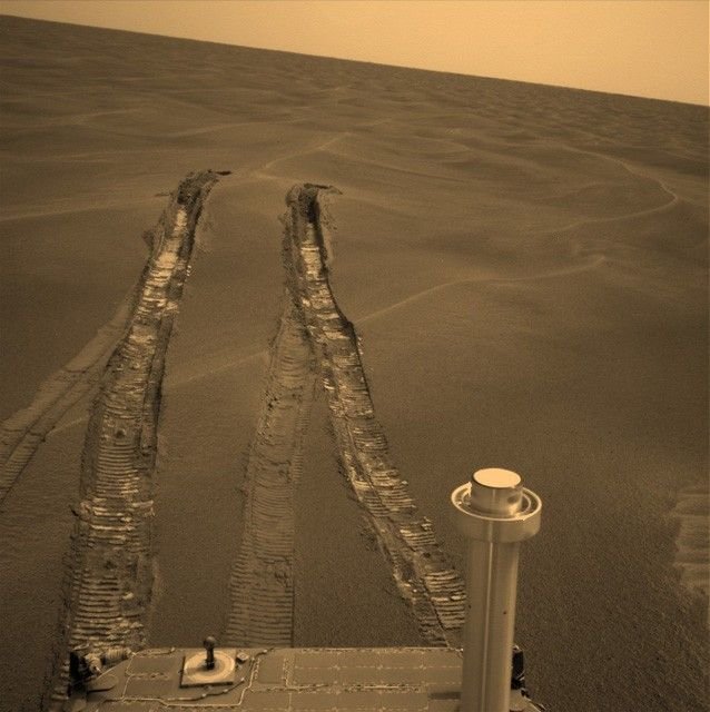
- Opportunity at “Purgatory Dune” (2005):
While traversing the Meridiani Planum, the Opportunity rover drove into a wind-ripple dune. The wheel encoders reported that the rover had traveled nearly 100 meters. In reality, due to the granular nature of the sand, the rover had barely moved a few centimeters. The slip ratio approached 100%. Had the rover been executing an autonomous blind drive based solely on wheel ticks, it would have believed it had reached its destination while actually digging its own grave. - Spirit at “Troy” (2009):
The Spirit rover became permanently embedded in soft soil because the crust broke under the rover’s weight. The mismatch between the commanded drive and the actual vehicle response (sinkage and high slip) led to the end of the mission’s mobile phase. - Curiosity at “Hidden Valley” (2014):
During its ascent to Mount Sharp, Curiosity encountered sand ripples that caused slip ratios to spike unexpectedly. The flight software, detecting a variance between the visual estimate and the wheel estimate, triggered a fault condition, stopping the rover to prevent it from sliding sideways into rocky hazards.
The Accumulation of Error (Drift)
Even without catastrophic events like Purgatory Dune, Dead Reckoning suffers from Integration Drift.
A seemingly negligible slip error of 2% might be acceptable over 10 meters. However, navigation errors are cumulative. Over a 1-kilometer drive, a 2% error results in a 20-meter positional discrepancy.
In the context of sample return missions (like the Mars Sample Return campaign), where a rover must revisit a specific location to pick up a sample tube with centimeter-level precision, a 20-meter error is unacceptable.
This inherent unreliability of mechanical odometry forces the navigation system to abandon the wheels as a source of truth and turn to the only sensor that can observe the environment directly: the camera.
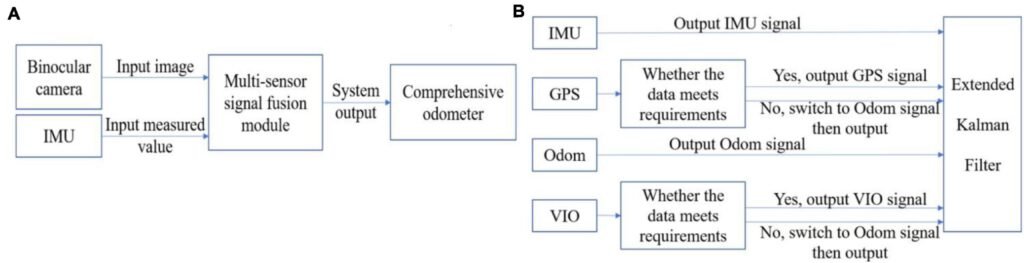
Sensor Fusion: Integrating VO with IMU (The EKF)
While Visual Odometry provides a geometric “truth,” it suffers from a critical weakness: it is computationally heavy. Processing stereo images takes time. On a processor like the RAD750, this might only happen once every few seconds. If the rover slips or drops off a small ledge between camera frames, Visual Odometry is effectively blind to that specific moment of motion.
To bridge these gaps, engineers fuse vision with the Inertial Measurement Unit (IMU)—the rover’s “inner ear.” The IMU is fast (hundreds of Hz) but prone to drift. The solution to balancing these two imperfect sensors is the Extended Kalman Filter (EKF).
Defining the Rover’s “State”
To the flight software, the rover is not a physical object; it is a State Vector (\mathbf{x}). This vector contains all the variables necessary to describe the rover’s motion in 3D space at any specific time step k.
In a typical Mars rover navigation stack, the state vector is a column matrix that tracks position, velocity, orientation (often as quaternions to avoid Gimbal Lock), and the critical IMU biases:
\mathbf{x}_k =
\begin{bmatrix}
\mathbf{p} \\
\mathbf{v} \\
\mathbf{q} \\
\mathbf{b}_a \\
\mathbf{b}_g
\end{bmatrix}
=
\begin{bmatrix}
x, y, z \\
v_x, v_y, v_z \\
q_0, q_1, q_2, q_3 \\
b_{ax}, b_{ay}, b_{az} \\
b_{gx}, b_{gy}, b_{gz}
\end{bmatrix}- \mathbf{p}, \mathbf{v}: Position and Velocity.
- \mathbf{q}: Orientation quaternion.
- \mathbf{b}_a, \mathbf{b}_g: Accelerometer and Gyroscope biases (the internal errors of the sensors).
The Matrix of Uncertainty (P)
The EKF does not just track where the rover is; it tracks how unsure it is about that location. This is represented by the Error Covariance Matrix (\mathbf{P}).
If \mathbf{x} has n elements (e.g., 15 states), \mathbf{P} is an n \times n matrix. The diagonal elements represent the variance (uncertainty) of each state variable, while the off-diagonal elements represent the correlations between them.
\mathbf{P}_k = \begin{bmatrix} \sigma^2_{p_x} & \dots & \rho_{p_x v_x} \\ \vdots & \ddots & \vdots \\ \rho_{v_x p_x} & \dots & \sigma^2_{b_{gz}} \end{bmatrix}When the rover relies solely on the IMU for a long period, the values in \mathbf{P} grow larger, indicating high uncertainty (“I think I’m here, but I could be 2 meters away”).
The Fusion: The Kalman Gain
The magic happens during the “Update Step.” When the Visual Odometry system successfully processes an image and outputs a new position measurement (\mathbf{z}_k), the EKF must decide how much to trust this new visual data versus its current IMU-based prediction.
This decision is governed by the Kalman Gain (\mathbf{K}). The gain matrix determines the “weight” given to the new visual information:
\mathbf{K}_k = \mathbf{P}_k^- \mathbf{H}^T (\mathbf{H} \mathbf{P}_k^- \mathbf{H}^T + \mathbf{R}_k)^{-1}- \mathbf{P}_k^-: The current uncertainty of the rover’s prediction.
- \mathbf{R}_k: The noise covariance of the Visual Odometry (how “noisy” the camera data is).
- \mathbf{H}: The measurement matrix mapping state to measurement space.
If the Visual Odometry is precise (low \mathbf{R}), the Kalman Gain \mathbf{K} increases, pulling the state vector \mathbf{x} strongly toward the visual measurement. If the rover is in a feature-poor environment and the VO is noisy (high \mathbf{R}), \mathbf{K} decreases, and the rover effectively ignores the visual data, sticking to its inertial prediction.
This matrix operation allows the rover to mathematically “negotiate” reality between its sensors, ensuring that the estimated position is always statistically optimal.
From “Stop-and-Go” to “Thinking-While-Driving”
The mathematical elegance of Visual Odometry (VO) comes with a heavy computational price. Solving the matrix inversions for the Extended Kalman Filter and calculating disparity maps requires millions of operations per second.
As we analyzed in our historical breakdown, The Evolution of Rover AI: From Sojourner’s ‘Bump and Go’ to Perseverance’s AutoNav, this computational load has historically been the primary bottleneck for Martian navigation.
The Legacy Bottleneck: Sequential Processing
For previous generations like Spirit and Opportunity, the onboard RAD6000 CPU simply could not process vision and drive simultaneously. The navigation logic was strictly sequential: move a meter, stop, snap photos, process the VO, and plan the next move.
This “Stop-and-Go” cycle drastically limited the effective average speed to roughly 10 meters per hour, despite the wheels being mechanically capable of moving faster. The rover wasn’t limited by its suspension, but by the speed of its thoughts.
The FPGA Leap: Hardware-Accelerated VO
The game changed with Perseverance and the introduction of AutoNav 2.0. Instead of relying on the main CPU (the RAD750) for vision, engineers offloaded the heavy lifting of Visual Odometry to a dedicated co-processor: the Vision Compute Element (VCE), powered by FPGAs (Field-Programmable Gate Arrays).
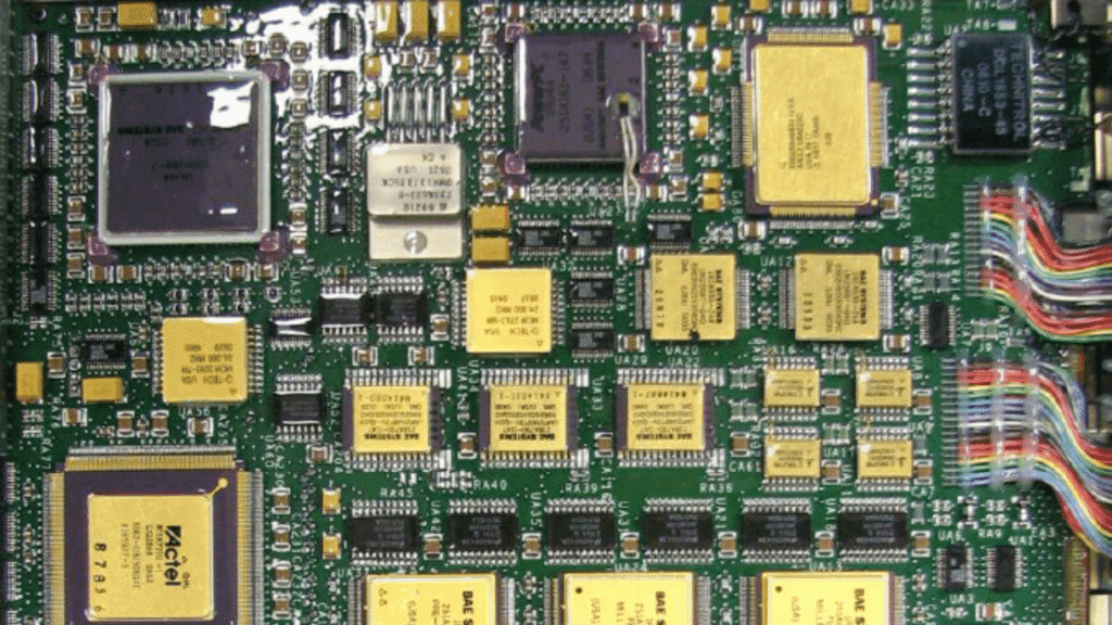
Unlike a standard CPU that executes instructions sequentially, FPGAs allow the VO algorithms—specifically stereo matching and image rectification—to be “printed” into the physical logic gates of the chip. This enables parallel processing:
- The FPGA handles the raw Visual Odometry pipeline in real-time.
- The CPU is free to focus on high-level path planning (A* Algorithm).
This architecture allows the rover to “Think-While-Driving,” processing navigation data while the wheels are in motion. The result is a six-fold increase in autonomous speed, reaching 120 meters per hour, essentially solving the latency problem through silicon specialization.
When VO Fails: The Geometric Hazard
Despite the sophistication of modern algorithms, Visual Odometry is not infallible. It relies on a fundamental assumption: the environment must be distinguishable. This creates a unique vulnerability known as Texture Starvation or Geometric Hazard.
In the context of Rover Perception, stereo vision performs poorly on uniform terrain, such as smooth sheets of sand or dust-covered flats. Without high-contrast features—sharp edges, rock shadows, or texture gradients—the feature extraction algorithms (like the FAST corner detector) cannot find unique points to track.
Perceptual Aliasing
A more insidious problem is Perceptual Aliasing. In vast dune fields, one patch of sand looks nearly identical to another. This high terrain self-similarity can trick the rover into associating its current view with the wrong reference frame. If the rover attempts to match features in a repetitive pattern, the mathematical solution for its motion becomes unstable. The “uncertainty” in the Kalman Filter spikes, indicating that the navigation solution is no longer trustworthy.
Fault Protection: The “Safe Mode”
So, what happens when the math breaks? The rover does not guess. Mission architects implement rigorous Fault Protection logic. If the Visual Odometry system fails to converge on a solution, or if the confidence interval (covariance) exceeds a safety threshold, the rover triggers a “Stop” command. This is the Digital Leash in action. The rover enters a Safe Mode, halting all motion and sending a telemetry alert to Earth. It effectively says, “I am blind; I will wait for instructions.” This conservative approach ensures that a 2.5-billion-dollar asset does not drive off a cliff due to a calculation error, prioritizing safety over speed.
Conclusion
To answer the question “How Rovers Know ‘How Far’ They’ve Gone”, we must look beyond the wheels. In the deceptive, high-slip environment of Mars, mechanical odometry is a liar. The truth is found in the Visual Odometry pipeline—a complex synthesis of linear algebra, feature tracking, and sensor fusion that allows a robot to “feel” its motion through its cameras.
However, Visual Odometry is just the beginning. As we explored in our deep dive into What is SLAM? How Rovers Map Alien Worlds in Real-Time, the future of exploration is moving from simple localization to Simultaneous Localization and Mapping (SLAM). While VO tells the rover where it is relative to where it started a moment ago, SLAM allows it to understand where it is on a global map, correcting drift over kilometers of travel.
This shift from reactive navigation to cognitive autonomy is not just an upgrade; it is a necessity for the future of space exploration. As humanity targets the “Ocean Worlds”—the icy moons of Europa and Titan—the communication latency will stretch from minutes to hours. In those dark, distant, and GPS-denied environments, there will be no “Safe Mode” calls to Earth for every small error. The next generation of rovers must not only know how far they have gone but understand where they are going, with absolute, independent certainty.

Lascia un commento